2D example: granular column collapse

By Yongjin Choi, Georgia Institute of Technology Website

import numpy as np 
import matplotlib.pyplot as plt
from tqdm import tqdm

Problem

This example considers a granular column collapse problem. The column is represented with material points and then subjected to a collapse due to gravity. The particles are modeled using the Drucker-Prager plasticity model.

Helper functions

def elasticity_matrix(youngs_modulus: float, poissons_ratio: float, stress_state: str) -> np.ndarray:
    """Compute the elasticity (stiffness) matrix for an isotropic elastic material.
    
    Args:
        youngs_modulus: Young's modulus of the material.
        poissons_ratio: Poisson's ratio of the material.
        stress_state: Type of stress state. Must be one of "PLANE_STRESS", 
                      "PLANE_STRAIN", or "3D".
    
    Returns:
        Elasticity matrix as a numpy array.
        
    Raises:
        ValueError: If an invalid stress_state is provided.
    """
    if stress_state == 'PLANE_STRESS':
        C = youngs_modulus / (1 - poissons_ratio**2) * np.array([
            [1, poissons_ratio, 0],
            [poissons_ratio, 1, 0],
            [0, 0, (1 - poissons_ratio) / 2]
        ])
    elif stress_state == 'PLANE_STRAIN':
        C = youngs_modulus / ((1 + poissons_ratio) * (1 - 2 * poissons_ratio)) * np.array([
            [1 - poissons_ratio, poissons_ratio, 0],
            [poissons_ratio, 1 - poissons_ratio, 0],
            [0, 0, 0.5 - poissons_ratio]
        ])
    else:  # 3D stress state
        C = np.zeros((6, 6))
        C[:3, :3] = youngs_modulus / ((1 + poissons_ratio) * (1 - 2 * poissons_ratio)) * np.array([
            [1 - poissons_ratio, poissons_ratio, poissons_ratio],
            [poissons_ratio, 1 - poissons_ratio, poissons_ratio],
            [poissons_ratio, poissons_ratio, 1 - poissons_ratio]
        ])
        C[3:, 3:] = youngs_modulus / (2 * (1 + poissons_ratio)) * np.eye(3)
    return C


def generate_rectangular_particles(origin, length, height, spacing):
    """
    Generate a numpy array that discretizes a rectangular shaped mass into equally spaced material points.
    
    Parameters:
    origin (tuple): (x, y) coordinates of the bottom left corner of the rectangle
    length (float): Length of the rectangle
    width (float): Width of the rectangle
    spacing (float): Distance between adjacent particles
    
    Returns:
    numpy.ndarray: Array of shape (n, 2) containing the coordinates of material points
    """
    
    # Calculate the number of points along each dimension
    nx = int(np.ceil(length / spacing)) + 1
    ny = int(np.ceil(height / spacing)) + 1
    
    # Generate equally spaced points along x and y axes
    x = np.linspace(origin[0], origin[0] + length, nx)
    y = np.linspace(origin[1], origin[1] + height, ny)
    
    # Create a mesh grid
    xx, yy = np.meshgrid(x, y)
    
    # Reshape the meshgrid into a 2D array of points
    points = np.column_stack((xx.ravel(), yy.ravel()))
    
    return points


def particle_element_mapping(particle_positions: np.ndarray, cell_width: float, cell_height: float,
                             n_ele_x: int, n_elements: int):
    """Map each particle to an element based on its position.
    
    Args:
        particle_positions: Particle positions as an array of shape (n_particles, 2).
        cell_width: Element (cell) width in the x-direction.
        cell_height: Element (cell) height in the y-direction.
        n_ele_x: Number of elements in the x-direction.
        n_elements: Total number of elements.
    
    Returns:
        ele_ids: Array of element ids for each particle.
        particle_ids_in_elements: List of particle indices for each element.
    """
    x_indices = np.floor(particle_positions[:, 0] / cell_width).astype(int)
    y_indices = np.floor(particle_positions[:, 1] / cell_height).astype(int)
    ele_ids = x_indices + n_ele_x * y_indices

    particle_ids_in_elements = [[] for _ in range(n_elements)]
    for p, e in enumerate(ele_ids):
        particle_ids_in_elements[e].append(p)

    return ele_ids, particle_ids_in_elements


def lagrange_basis(element_type: str, local_coord: np.ndarray):
    """Compute the shape functions and their derivatives for a finite element.
    
    Args:
        element_type: Type of element. Currently only "Q4" is supported.
        local_coord: Array of local coordinates [xi, eta].
    
    Returns:
        N: Shape function values.
        dN_dxi: Derivatives of the shape functions with respect to xi and eta.
        
    Raises:
        ValueError: If an unsupported element type is provided.
    """
    if element_type == 'Q4':
        xi, eta = local_coord
        N = np.array([
            (1 - xi) * (1 - eta),
            (1 + xi) * (1 - eta),
            (1 + xi) * (1 + eta),
            (1 - xi) * (1 + eta)
        ]) / 4.0

        dN_dxi = np.array([
            [-(1 - eta), -(1 - xi)],
            [ (1 - eta), -(1 + xi)],
            [ (1 + eta),  (1 + xi)],
            [-(1 + eta),  (1 - xi)]
        ]) / 4.0
    else:
        raise ValueError(f"Unsupported element type: {element_type}")

    return N, dN_dxi


def compute_local_coord(particle_pos: np.ndarray, element_coords: np.ndarray,
                        cell_width: float, cell_height: float) -> np.ndarray:
    """Compute the local (ξ, η) coordinates for a particle within an element.
    
    Args:
        particle_pos: [x, y] coordinates of the particle.
        element_coords: Coordinates of the element nodes (4 x 2 array).
        cell_width: Element width in the x-direction.
        cell_height: Element height in the y-direction.
    
    Returns:
        Local coordinates [ξ, η].
    """
    xi = (2 * particle_pos[0] - (element_coords[0, 0] + element_coords[1, 0])) / cell_width
    eta = (2 * particle_pos[1] - (element_coords[1, 1] + element_coords[2, 1])) / cell_height
    return np.array([xi, eta])

import numpy as np
import matplotlib.pyplot as plt
import matplotlib.cm as cm

# Temporary hard-coded variable
nu = 0.3

def principal_stresses(stress_tensor):
    """
    Calculate the principal stresses sigma_1 and sigma_2 for a 2D stress tensor using eigen decomposition.

    Parameters:
    stress_tensor (list): A list of the form [sigma_xx, sigma_yy, sigma_xy].

    Returns:
    tuple: Principal stresses (sigma_1, sigma_2) with sigma_1 >= sigma_2.
    """
    # Unpack the stress components
    sigma_xx, sigma_yy, sigma_xy = stress_tensor

    # Form the 2D stress tensor matrix
    stress_matrix = np.array([[sigma_xx, sigma_xy],
                              [sigma_xy, sigma_yy]])

    # Perform eigen decomposition to get the eigenvalues (principal stresses)
    eigenvalues, _ = np.linalg.eig(stress_matrix)

    # Sort eigenvalues in descending order: sigma_1 >= sigma_2
    sigma_1, sigma_2 = np.sort(eigenvalues)[::-1]

    return sigma_1, sigma_2


# Function to compute alpha and k from friction angle and cohesion
def drucker_prager_parameters(friction_angle_deg, cohesion):
    # Convert friction angle to radians
    phi = np.radians(friction_angle_deg)
    
    # Compute alpha and k
    alpha = (2 * np.sin(phi)) / (np.sqrt(3) * (3 - np.sin(phi)))
    # alpha = 0
    k = (6 * cohesion * np.cos(phi)) / (np.sqrt(3) * (3 - np.sin(phi)))
    
    return alpha, k

# Elasticity matrix (2D plane strain assumption)
def elasticity_matrix(E, nu):
    D = (E / ((1 + nu) * (1 - 2 * nu))) * np.array([
        [1 - nu,     nu,          0],
        [nu,         1 - nu,      0],
        [0,          0,           (1 - 2 * nu) / 2]
    ])
    return D

# Invariants of the stress tensor
def compute_invariants(stress, stress_condition="plane_strain"):
    sigma_xx, sigma_yy, tau_xy = stress
    
    if stress_condition != "plane_strain":
        # First invariant
        I1 = sigma_xx + sigma_yy  
        
        # J2 invariant
        # Deviatoric stresses
        s_xx = sigma_xx - I1 / 2
        s_yy = sigma_yy - I1 / 2
        s_xy = tau_xy
        
        # J2 = 0.5 * s:s
        J2 = 0.5 * (s_xx**2 + s_yy**2 + s_xy**2)
        # The above is equivalent to:
        # J2 = (1/4) * (sigma_x - sigma_y)**2 + tau_xy**2
        
    else:  # Plain strain constraint
        sigma_zz = nu * (sigma_xx + sigma_yy)
        I1 = sigma_xx + sigma_yy + sigma_zz
        
        # Deviatoric stresses
        s_xx = sigma_xx - I1 / 3
        s_yy = sigma_yy - I1 / 3
        s_zz = sigma_zz - I1 / 3
        s_xy = tau_xy
        
        # J2 = 0.5 s:s
        J2 = 0.5 * (s_xx**2 + s_yy**2 + s_zz**2 + s_xy**2)
    
    return I1, J2

# Drucker-Prager yield function
def drucker_prager_yield(stress, alpha, k):
    I1, J2 = compute_invariants(stress)
    return alpha * I1 + np.sqrt(J2) - k

# Gradient of yield function df/dsigma
def df_dsigma(stress, alpha):
    sigma_x, sigma_y, tau_xy = stress
    I1, J2 = compute_invariants(stress)
    
    dfdx = alpha + (sigma_x - sigma_y) / np.sqrt(J2)
    dfdy = alpha - (sigma_x - sigma_y) / np.sqrt(J2)
    dftau = 2 * tau_xy / np.sqrt(J2)
    return np.array([dfdx, dfdy, dftau])

# Update stress and strain process
def update_stress_strain(stress_n, strain_n, strain_increment, D, alpha, k):
    # Step 1: Compute trial stress
    stress_trial = stress_n + np.dot(D, strain_increment)
    
    # Step 2: Check yield condition
    f_trial = drucker_prager_yield(stress_trial, alpha, k)
    # print(f_trial)
    
    if f_trial <= 0:
        # Elastic step: no plastic deformation
        return stress_trial, strain_n + strain_increment, 0.0  # No plastic multiplier
    
    # Step 3: Plastic step - compute the plastic multiplier Δλ
    df_sigma = df_dsigma(stress_trial, alpha)
    
    H = np.dot(df_sigma, np.dot(D, df_sigma))
    delta_lambda = f_trial / H
    
    # Step 4: Update stress using the return mapping scheme
    stress_updated = stress_trial - delta_lambda * np.dot(D, df_sigma)
    # stress_updated[1] = 100  # yc: keep sigma_y constant for triaxial test
    
    # Step 5: Update plastic strain
    plastic_strain_increment = delta_lambda * df_sigma
    strain_updated = strain_n + plastic_strain_increment
    
    return stress_updated, strain_updated, delta_lambda

Material properties

# Material properties
E = 100000
nu = 0.3
rho = 3600
mu = 0.385
phi = 30
c = 1
K0 = 0.5

Analysis setting

# Analysis setting
dtime = 0.0001
time = 1.0
t = 0
interval = 200
g = 4.8

Mesh generation

# length of domain
l = 1

# number of elements for each dim
n_ele_x = 20
n_ele_y = 20

# cell size
delta_x = l / n_ele_x
delta_y = l / n_ele_y

# number of grid nodes
n_node_x = n_ele_x + 1
n_node_y = n_ele_y + 1
n_nodes = n_node_x * n_node_y

# Generate mesh nodes
x_coords = np.linspace(0, l, n_node_x)
y_coords = np.linspace(0, l, n_node_y)
X, Y = np.meshgrid(x_coords, y_coords)
nodes = np.vstack([X.flatten(), Y.flatten()]).T

# Generate elements (connectivity)
elements = []
for j in range(n_node_y - 1):
    for i in range(n_node_x - 1):
        n1 = j * n_node_x + i
        n2 = n1 + 1
        n3 = n2 + n_node_x
        n4 = n1 + n_node_x
        elements.append([n1, n2, n3, n4])
elements = np.array(elements)
elements_coordinate_map = nodes[elements]
n_elements = elements.shape[0]

# Boundary nodes
bottomNodes = np.where(nodes[:, 1] < 1e-8)[0]
upperNodes = np.where(nodes[:, 1] > l - 1e-8)[0]
leftNodes = np.where(nodes[:, 0] < 1e-8)[0]
rightNodes = np.where(nodes[:, 0] > l - 1e-8)[0]

# Initialize node quantities
n_masses = np.zeros(n_nodes)  # nodal masses
n_momentums = np.zeros((n_nodes, 2))  # nodal momentums
n_iforces = np.zeros((n_nodes, 2))  # Internal forces
n_eforces = np.zeros((n_nodes, 2))  # External forces. Not used in this practice
# Initialize grid state variables
gStress = np.zeros((3, n_nodes))  # [sig_xx, sig_yy, sig_xy]
gDisp = np.zeros((2, n_nodes))  # [disp_x, disp_y]

Generate particles

# Inputs for particles representing granular column
origin = [0.0125, 0.0125]
lengths = [0.300, 0.300]
n_particle_per_cell_per_dim = 2

# Generate particles for granular column body
spacing = delta_x / n_particle_per_cell_per_dim
xp = generate_rectangular_particles(
    origin=origin, length=lengths[0], height=lengths[1], spacing=spacing)

# particle states
vp = np.zeros(xp.shape)
s = np.zeros((len(xp), 3))  # [sigma_xx, sigma_yy, sigma_xy]
eps = np.zeros((len(xp), 3))  # [epsilon_xx, epsilon_yy, gamma_xy]
Fp = np.tile([1.0, 0.0, 0.0, 1.0], (len(xp), 1))

# Find elements to which particles belong
ele_ids_of_particles, p_ids_in_eles = particle_element_mapping(
    xp, delta_x, delta_y, n_ele_x, n_elements)
active_elements = np.unique(ele_ids_of_particles)
active_nodes = np.unique(elements[active_elements, :])

# Compute initial particle volume
Vp = np.zeros(len(xp))
# Volume (area) of each background cell
for p_ids_in_ele in p_ids_in_eles:
    n_mp_in_element = len(p_ids_in_ele)
    if n_mp_in_element > 0:
        volume_per_mp = (delta_x * delta_y) / n_mp_in_element
        Vp[p_ids_in_ele] = volume_per_mp
Vp0 = Vp.copy()  # save initial volume
Mp = Vp * rho  # mass of particles

# Initialize stress
height = lengths[1] + spacing / 2
s[:, 1] = - g * rho * (height - xp[:, 1])
s[:, 0] = K0 * s[:, 1]

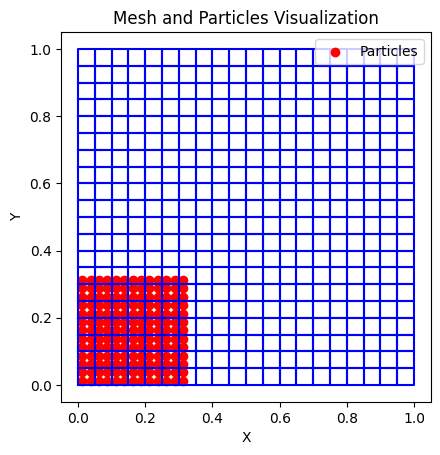
# Plot mesh, particles
meshes = [(nodes, elements)]
def plot_mesh_and_particles(nodes, elements, particles):
    fig, ax = plt.subplots()

    # Plot the mesh
    for element in elements:
        # Get the coordinates of the element's nodes
        quad_coords = nodes[element]
        # Repeat the first point to close the quad
        quad_coords = np.vstack([quad_coords, quad_coords[0]])
        ax.plot(quad_coords[:, 0], quad_coords[:, 1], 'b-', linewidth=1.5)  # Blue lines for the mesh

    # Plot the particles
    ax.scatter(particles[:, 0], particles[:, 1], color='red', marker='o', label='Particles')

    # Set labels and title
    ax.set_xlabel('X')
    ax.set_ylabel('Y')
    ax.set_title('Mesh and Particles Visualization')
    ax.legend()

    # Equal aspect ratio
    ax.set_aspect('equal', 'box')

    plt.show()
plot_mesh_and_particles(nodes, elements, xp)

Run analysis

# Results to save
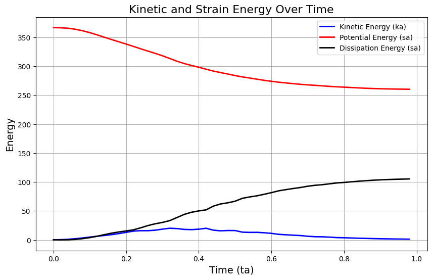
ta = []  # time
ka = []  # kinetic energy
pa = []  # potential energy
da = []  # dissipation energy
# sa = []  # strain energy
pos = []  # positions
vel = []  # velocities
stresses = []
strains = []

nsteps = int(time / dtime)

istep = 0
potential_e_t0 = np.sum(Mp * g *  xp[:, 1])


for istep in tqdm(range(nsteps), desc="Simulating"):
    # print(f"Time: {t:.5f}/{time}")
    
    # Compute potential energy
    potential_e = np.sum(Mp * g *  xp[:, 1])
    kinetic_e = np.sum(0.5 * Mp * np.linalg.norm(vp, axis=1)**2)
    dissipation_e = potential_e_t0 - kinetic_e - potential_e

    # Refresh the nodal values
    n_masses.fill(0)
    n_momentums.fill(0)
    n_iforces.fill(0)
    n_eforces.fill(0)
    gStress.fill(0)
    
    # Iterate over the computational cells (i.e., elements)
    for ele_id in active_elements:
        # node ids of the current element
        node_ids = elements[ele_id]
        # coords of the current element
        node_coords = nodes[node_ids, :]  
        # particle ids inside the current element
        material_points = p_ids_in_eles[ele_id]

        # Iterate over the material points in the current cell
        for p in material_points:
            
            # Convert global coordinate "p=(x, y)" to local coordiate "pt=(xi, eta)".
            pt = np.array(
                [(2 * xp[p, 0] - (node_coords[0, 0] + node_coords[1, 0])) / delta_x,
                 (2 * xp[p, 1] - (node_coords[1, 1] + node_coords[2, 1])) / delta_y])

            # Evaluate shape function and its derivatives with respect to local coords (xi, eta) at (x, y).
            N, dNdxi = lagrange_basis("Q4", pt)
            # Evaluate the Jacobian at current the current local coords (xi, eta).
            J0 = node_coords.T @ dNdxi
            # Get the inverse of Jacobian
            invJ0 = np.linalg.inv(J0)
            # Get the derivative of shape function with respect to global coords, i.e., (x, y)
            dNdx = dNdxi @ invJ0

            # Current stress of material points
            stress = s[p, :]
            
            # Iterate over the nodes of the current element & update nodal values by interpolating material point values
            for i, node_id in enumerate(node_ids):
                dNIdx = dNdx[i, 0]
                dNIdy = dNdx[i, 1]
                n_masses[node_id] += N[i] * Mp[p]
                n_momentums[node_id, :] += N[i] * Mp[p] * vp[p, :]
                n_iforces[node_id, 0] -= Vp[p] * (stress[0] * dNIdx + stress[2] * dNIdy)
                n_iforces[node_id, 1] -= Vp[p] * (stress[2] * dNIdx + stress[1] * dNIdy)
                n_eforces[node_id, 1] -= N[i] * Mp[p] * g

    # Total nodal force
    nforce = n_iforces + n_eforces
    
    # Compute nodal accelerations
    n_accelerations = np.zeros((n_nodes, 2))
    # valid_mass = n_masses > 1e-12
    # n_accelerations[valid_mass, :] = nforce[valid_mass, :] / n_masses[valid_mass, None]
    n_accelerations[active_nodes, :] = nforce[active_nodes, :] / n_masses[active_nodes, None]
    
    
    # Boundary conditions
    # 0. Update nodal kinematics (nodal mass, momentum -> particles)
    # 1. Velocity & acceleration to 0
    # 2. Compute nodal force.
    #   * First, map particle body force to nodal body force
    #   * Next, map particle internal force to nodel internal force
    # 3. compute_particle_kinematics.
    #   * compute_acceleration_velocity
    #       * accel = (f_e + f_i) / mass
    #       * apply_friction_constraints
    #       * vel += accel * dt
    #       * apply_velocity_constraints
    #   * compute_updated_position
    
    
    # Function to apply frictional boundary condition on given nodes
    def apply_frictional_boundary_condition(node_ids, dir_n, sign_dir_n):
        dir_t = 1 - dir_n  # Tangential direction

        # Normal and tangential accelerations
        acc_n = n_accelerations[node_ids, dir_n]
        acc_t = n_accelerations[node_ids, dir_t]

        # Tangential velocities
        vel_t = n_momentums[node_ids, dir_t] / n_masses[node_ids]

        # Determine nodes where particles are acting towards the boundary
        positive_movement_towards_boundary = (acc_n * sign_dir_n) > 0.0

        # Apply frictional boundary condition
        for idx in np.where(positive_movement_towards_boundary)[0]:
            node_id = node_ids[idx]
            acc_n_i = acc_n[idx]
            acc_t_i = acc_t[idx]
            vel_t_i = vel_t[idx]
            # print(vel_t_i)
            
            # Determine static or kinetic friction
            if vel_t_i != 0.0:  # Kinetic friction
                # compute tangential velocity at next timestep
                vel_net = dtime * acc_t_i + vel_t_i
                vel_frictional = dtime * mu * abs(acc_n_i)
                if abs(vel_net) <= vel_frictional:
                    # friction stops the particle
                    acc_t_i = -vel_t_i / dtime
                else:
                    # friction reduces the tangential acceleration
                    acc_t_i -= np.sign(vel_net) * mu * abs(acc_n_i)
                # acc_t_i -= np.sign(vel_net) * mu * abs(acc_n_i)
            else:  # Static friction
                if abs(acc_t_i) <= mu * abs(acc_n_i):
                    acc_t_i = 0.0
                else:
                    acc_t_i -= np.sign(acc_t_i) * mu * abs(acc_n_i)

            # Update tangential acceleration
            n_accelerations[node_id, dir_t] = acc_t_i

            # Update nodal force at this node
            nforce[node_id, :] = n_accelerations[node_id, :] * n_masses[node_id]
    
    apply_frictional_boundary_condition(
        np.intersect1d(leftNodes, active_nodes), dir_n=0, sign_dir_n=-1.0)
    apply_frictional_boundary_condition(
        np.intersect1d(rightNodes, active_nodes), dir_n=0, sign_dir_n=1.0)
    apply_frictional_boundary_condition(
        np.intersect1d(bottomNodes, active_nodes), dir_n=1, sign_dir_n=-1.0)
    apply_frictional_boundary_condition(
        np.intersect1d(upperNodes, active_nodes), dir_n=1, sign_dir_n=1.0)
    
    # Impose boundary condition
    n_momentums[leftNodes, 0] = 0
    n_momentums[rightNodes, 0] = 0
    n_momentums[bottomNodes, 1] = 0
    n_momentums[upperNodes, 1] = 0
    nforce[leftNodes, 0] = 0
    nforce[rightNodes, 0] = 0
    nforce[bottomNodes, 1] = 0
    nforce[upperNodes, 1] = 0
    
    # Update nomal momentum
    n_momentums += nforce * dtime    
    
    k = 0
    u = 0
    
    # Iterate over the computational cells (i.e., elements)
    for ele_id in active_elements:
        # node ids of the current element
        node_ids = elements[ele_id]
        # coords of the current element
        node_coords = nodes[node_ids, :]  
        # particle ids inside the current element
        material_points = p_ids_in_eles[ele_id]

        # Iterate over the material points in the current cell
        for p in material_points:
            # Convert global coordinate "p=(x, y)" to local coordiate "pt=(xi, eta)".
            pt = np.array(
                [(2 * xp[p, 0] - (node_coords[0, 0] + node_coords[1, 0])) / delta_x,
                 (2 * xp[p, 1] - (node_coords[1, 1] + node_coords[2, 1])) / delta_y])

            N, dNdxi = lagrange_basis("Q4", pt)
            J0 = node_coords.T @ dNdxi
            invJ0 = np.linalg.inv(J0)
            dNdx = dNdxi @ invJ0
            Lp = np.zeros((2, 2))
            
            for i, node_id in enumerate(node_ids):  
                vI = np.zeros(2)
                vp[p, :] += dtime * N[i] * nforce[node_id, :] / n_masses[node_id]
                xp[p, :] += dtime * N[i] * n_momentums[node_id, :] / n_masses[node_id]
                vI = n_momentums[node_id, :] / n_masses[node_id]  # nodal velocity
                Lp += vI.reshape(2, 1) @ dNdx[i, :].reshape(1, 2)  # particle velocity gradient

            F = Fp[p, :].reshape(2, 2) @ (np.eye(2) + Lp * dtime)
            Fp[p, :] = F.flatten()
            Vp[p] = np.linalg.det(F) * Vp0[p]
            dEps = dtime * 0.5 * (Lp + Lp.T)
            
            D = elasticity_matrix(E, nu)
            alpha, k = drucker_prager_parameters(phi, c)
            new_sig, new_epsE, _ = update_stress_strain(
                stress_n=s[p, :],
                strain_n=eps[p, :],
                strain_increment=np.array([dEps[0, 0], dEps[1, 1], dEps[0, 1]]),
                D=D,
                alpha=alpha,
                k=k)

            s[p, :] = new_sig
            eps[p, :] = new_epsE

            for i, node_id in enumerate(node_ids):
                gStress[:, node_id] += N[i] * s[p, :]

    stresses.append(s.copy())
    strains.append(eps.copy())
    pos.append(xp.copy())
    vel.append(vp.copy())
    
    # Update particle-element mapping (elements to which particles belong)
    ele_ids_of_particles, p_ids_in_eles = particle_element_mapping(
        xp, delta_x, delta_y, n_ele_x, n_elements)
    active_elements = np.unique(ele_ids_of_particles)
    active_nodes = np.unique(elements[active_elements, :])

    if istep % interval == 0:
        # result = {"positions": xp, "stress": s}
        # save_dir = f"./results_vtk_column/"
        # visualizer.save_vtk(istep, result, save_dir)
        
        ta.append(t)
        ka.append(kinetic_e)
        pa.append(potential_e)
        da.append(dissipation_e)

        
    t += dtime
# Plot kinetic and strain energy
plt.figure(figsize=(10, 6))
plt.plot(ta, ka, label='Kinetic Energy (ka)', color='b', linewidth=2)
plt.plot(ta, pa, label='Potential Energy (sa)', color='r', linewidth=2)
plt.plot(ta, da, label='Dissipation Energy (sa)', color='k', linewidth=2)
plt.xlabel('Time (ta)', fontsize=14)
plt.ylabel('Energy', fontsize=14)
plt.title('Kinetic and Strain Energy Over Time', fontsize=16)
plt.legend()
plt.grid(True)
plt.show()

Simulating: 100%|██████████| 10000/10000 [03:12<00:00, 52.00it/s]

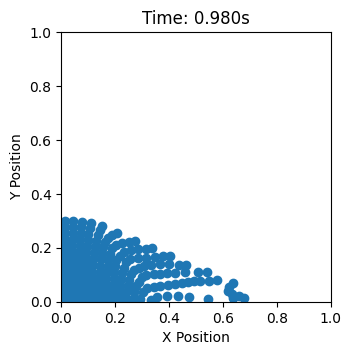
Visualize trajectory

from matplotlib.animation import FuncAnimation
from IPython.display import HTML

# Create figure and axis
fig, ax = plt.subplots(figsize=(5, 3.5))
ax.set_xlim(0, l)
ax.set_ylim(0, l)
ax.set_xlabel('X Position')
ax.set_ylabel('Y Position')
ax.set_title('Granular Column Collapse')

# Initialize scatter plot
scatter = ax.scatter([], [])

# Animation update function
def update(frame):
    scatter.set_offsets(pos[frame * interval])
    ax.set_title(f'Time: {ta[frame]:.3f}s')
    ax.set_aspect('equal')
    return scatter,

# Create animation
# Using the same interval as your save interval
anim = FuncAnimation(
    fig, update, 
    frames=len(ta),  # number of frames matches saved timesteps
    interval=50,     # 50ms between frames
    blit=True
)

# Display animation in notebook
HTML(anim.to_jshtml())

Once Loop Reflect

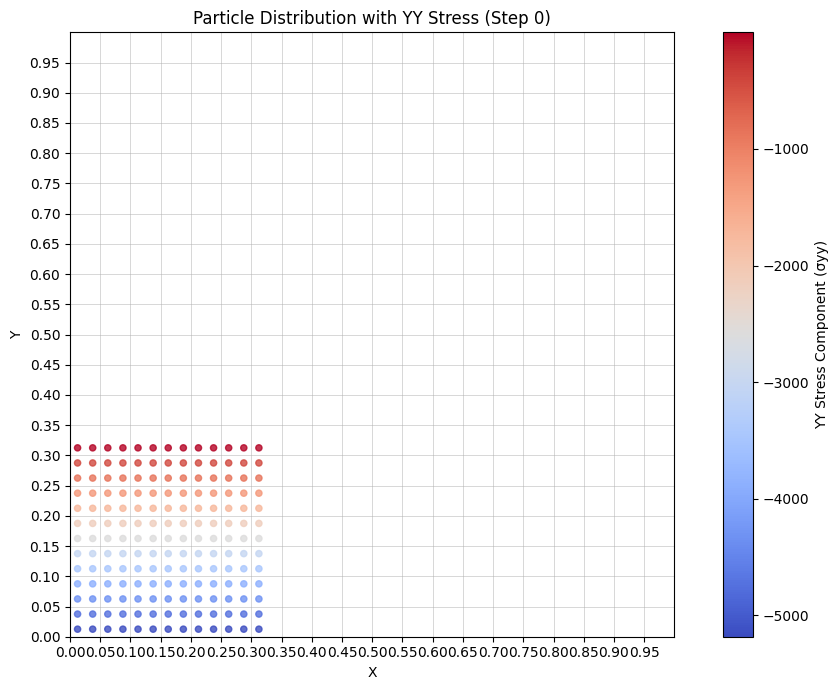
Visualize stress

# Create animation of particles colored by yy stress
fig, ax = plt.subplots(figsize=(10, 7))

# Set axis properties
ax.set_aspect('equal')
ax.set_xlabel('X')
ax.set_ylabel('Y')
ax.set_title('Particle Distribution with YY Stress')
ax.grid(True)

# Set fixed axis limits based on domain size
ax.set_xlim(0, l)
ax.set_ylim(0, l)

# Create a normalized colormap - use consistent limits for better visualization
vmin = min([np.min(stresses[0][:, 1]) for i in range(len(stresses))])
vmax = max([np.max(stresses[0][:, 1]) for i in range(len(stresses))])

# Create a ScalarMappable for the colorbar outside the animation function
sm = plt.cm.ScalarMappable(cmap='coolwarm', norm=plt.Normalize(vmin=vmin, vmax=vmax))
sm.set_array([])  # You need to set an array (empty in this case)
cbar = plt.colorbar(sm, ax=ax)
cbar.set_label('YY Stress Component (σyy)')

def update_stress_plot(frame):
    # Clear previous frame
    ax.clear()
    
    # Get yy stress component (s[:, 1]) for current frame
    yy_stress = stresses[frame * interval][:, 1]
    
    # Plot particles colored by stress
    scatter = ax.scatter(
        pos[frame * interval][:, 0], 
        pos[frame * interval][:, 1],
        c=yy_stress, 
        cmap='coolwarm', 
        vmin=vmin,
        vmax=vmax,
        s=20,
        alpha=0.8
    )
    
    # Set axis properties
    ax.set_aspect('equal')
    ax.set_xlabel('X')
    ax.set_ylabel('Y')
    ax.set_title(f'Particle Distribution with YY Stress (Step {frame * interval})')
    ax.grid(True)
    ax.grid(True, linestyle='-', linewidth=0.5, alpha=0.7)
    ax.set_xticks(np.arange(0, l, l/n_ele_x)) 
    ax.set_yticks(np.arange(0, l, l/n_ele_y)) 

    # Set fixed axis limits based on domain size
    ax.set_xlim(0, l)
    ax.set_ylim(0, l)
    plt.tight_layout()
    
    return scatter,

# Create animation
from matplotlib.animation import FuncAnimation

anim = FuncAnimation(
    fig, 
    update_stress_plot, 
    frames=len(ta),
    interval=100,  # milliseconds between frames
    blit=False
)

# Display the animation in the notebook
from IPython.display import HTML
HTML(anim.to_jshtml())

Once Loop Reflect

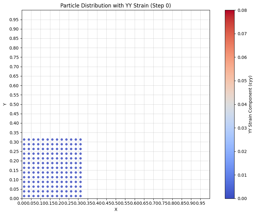
Visualize strain

# Create animation of particles colored by yy strain
fig, ax = plt.subplots(figsize=(10, 7))

# Set axis properties
ax.set_aspect('equal')
ax.set_xlabel('X')
ax.set_ylabel('Y')
ax.set_title('Particle Distribution with YY Strain')
ax.grid(True)

# Set fixed axis limits based on domain size
ax.set_xlim(0, l)
ax.set_ylim(0, l)

# Create a normalized colormap - use consistent limits for better visualization
vmin = 0
vmax = 0.08

# Create a ScalarMappable for the colorbar outside the animation function
sm = plt.cm.ScalarMappable(cmap='coolwarm', norm=plt.Normalize(vmin=vmin, vmax=vmax))
sm.set_array([])  # You need to set an array (empty in this case)
cbar = plt.colorbar(sm, ax=ax)
cbar.set_label('YY Strain Component (εyy)')

def update_strain_plot(frame):
    # Clear previous frame
    ax.clear()
    
    # Get yy strain component (eps[:, 1]) for current frame
    xy_strain = strains[frame * interval][:, 2]
    
    # Plot particles colored by strain
    scatter = ax.scatter(
        pos[frame * interval][:, 0], 
        pos[frame * interval][:, 1],
        c=xy_strain, 
        cmap='coolwarm', 
        vmin=vmin,
        vmax=vmax,
        s=20,
        alpha=0.8
    )
    
    # Set axis properties
    ax.set_aspect('equal')
    ax.set_xlabel('X')
    ax.set_ylabel('Y')
    ax.set_title(f'Particle Distribution with YY Strain (Step {frame * interval})')
    ax.grid(True)
    ax.grid(True, linestyle='-', linewidth=0.5, alpha=0.7)
    ax.set_xticks(np.arange(0, l, l/n_ele_x)) 
    ax.set_yticks(np.arange(0, l, l/n_ele_y)) 

    # Set fixed axis limits based on domain size
    ax.set_xlim(0, l)
    ax.set_ylim(0, l)
    plt.tight_layout()
    
    return scatter,

# Create animation
from matplotlib.animation import FuncAnimation

strain_anim = FuncAnimation(
    fig, 
    update_strain_plot, 
    frames=len(ta),
    interval=100,  # milliseconds between frames
    blit=False
)

# Display the animation in the notebook
from IPython.display import HTML
HTML(strain_anim.to_jshtml())

Once Loop Reflect